GIS and Remote Sensing in Geosciences

Lesson 3: GIS-supported modelling of mass movements

1. Modelling of mass movements and GIS

Nowadays, computer models in combination with GIS play a prominent role in the analysis of landslide hazards. A variety of approaches and tools is available for the computation of the release and propagation of mass movements. Specific methods are suitable for specific purposes, and modelling has to be combined with other types of investigation in order to get a complete picture. This lecture shall introduce some examples as well as challenges concerning the simulation of landslide propagation, whereas landslide release modelling will be covered in the training part of the lesson.

Download presentation GIS-based simulation of landslide processes

2. Definition of the specific problem

The slopes of the Mendoza Valley (Western Argentina) near the station of Guido are steep and the rock and debris slopes are susceptible to produce mass movements. Besides rock fall, shallow translational slope failures converting into debris flows are of particular interest. Such processes have repeatedly interfered with the important international road running through the valley. In order to take adequate measures, it is important to know in which places mass movement processes are likely to occur. GIS and RS can help to identify such areas. The delineation of potential onset areas of shallow landslides shall be a first step.

3. Retrieval and preparation of data

The lesson will be based on a 5 m DEM mv_elev.asc derived from a stereo pair of aerial images, a soil map mv_soilclass.shp, a land cover map mv_lcovclass.shp and two data tables mv_soilclass.txt and mv_lcovclass.txt assigning physical and geotechnical parameters to each soil and land cover class, according to laboratory tests and data from the literature. The polygons of mv_init.shp represent observed areas of slope instability. In addition, a Landsat TM image mv_landsat.img is provided in order to allow a visual impression of the training area. All data are prepared in a way to be usable for the analysis tasks without much preprocessing. Please consult Lesson 1 to learn how to prepare GIS data for analysis.

Access GIS and RS data sources
Download training data for the Mendoza Valley

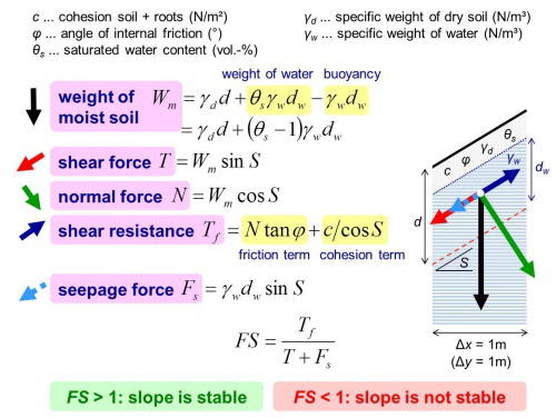
4. Slope stability modelling with infinite slope stability model

As shown in the first part of this lesson, the infinite slope stability model is particularly suitable for identifying areas susceptible to shallow translational failures of relatively uniform slopes. They are often used in combination with GIS since they build on a simple static relationship and do not require complex cell neighbourhood computations: the stability of a slope can easily be computed independently for each raster cell. Before starting, we have to prepare the required slope, geotechnical, hydraulic and land cover maps:

The DEM is provided in the ASCII format facilitating data exchange between different software packages (e.g., GRASS GIS and ArcGIS). Even though this format can be read by ArcGIS directly, it is better to properly import it to the ESRI Raster format. When working with GRASS GIS, the raster has to be converted to the GRASS raster format.
Learn how to import an ASCII Raster to GRASS GIS 6.4, to ArcGIS 9.3 and to ArcGIS 10

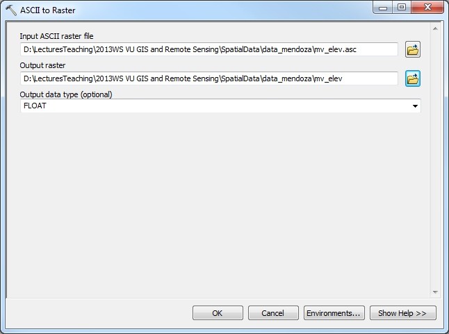
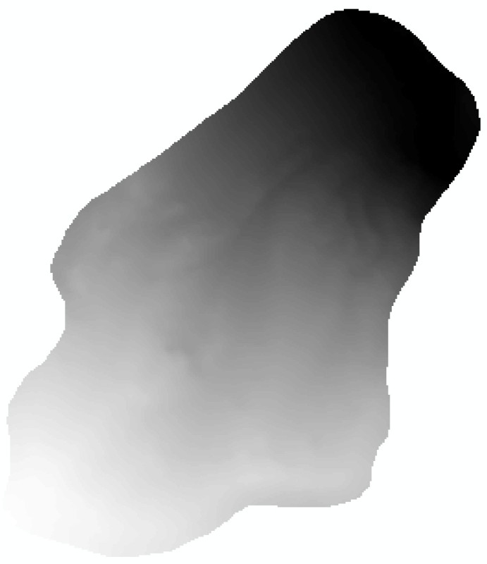
Import of the DEM provided as an ascii raster to an ESRI raster - dialog box (left) and result (right).
Derive slope and hillshade rasters from the DEM as you have learned it in the previous lessons.

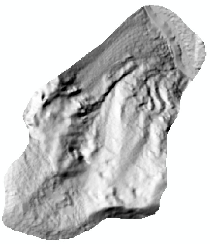
Slope (left) and hillshade (right).
Join the soil data table mv_soilclass.txt to the soil class map mv_soilclass.shp, using the CLASS column as identifier.
Learn how to join tables to vector layers in ArcGIS 9.3 and in ArcGIS 10

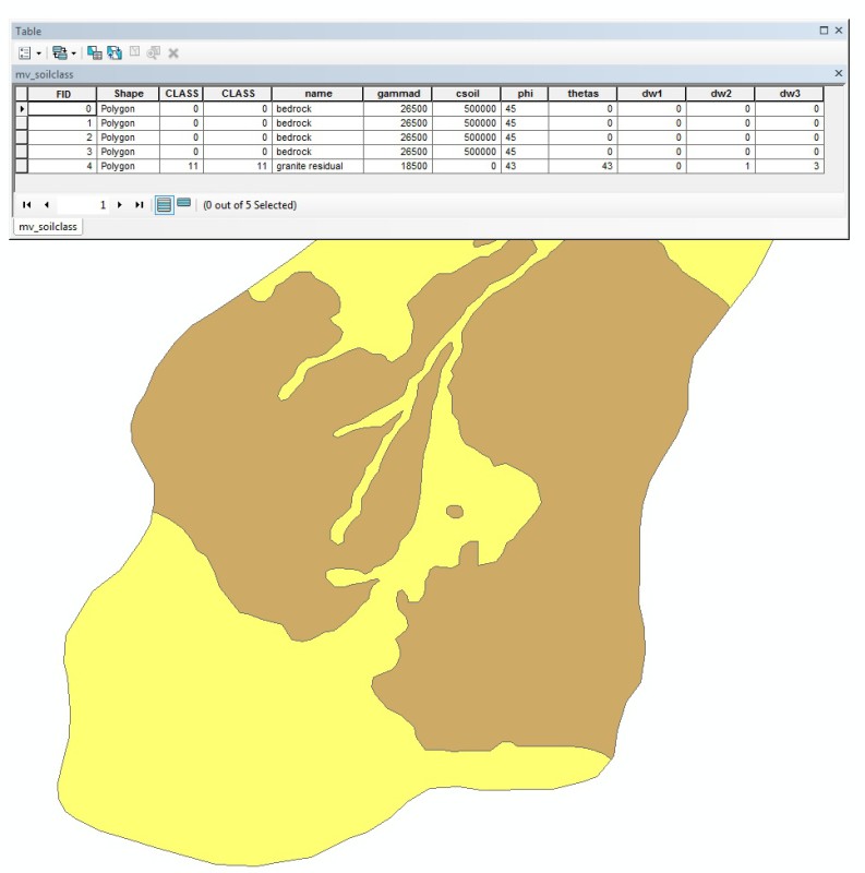
Joining the data assigned to each soil class to the attribute table of the soil class map.
Then, export the soil class map to a new shapefile in order to permanantly store the joined columns to the attribute table of the soil class map. Prepare raster maps of angle of internal friction φ, soil cohesion c_soil, dry soil specific weight γ_d, dry soil specific weight θ_s and saturated depths d_w,1, d_w,2 and d_w,3 from the polygons with the joined table.
Learn how to convert features to rasters in ArcGIS 9.3 and in ArcGIS 10

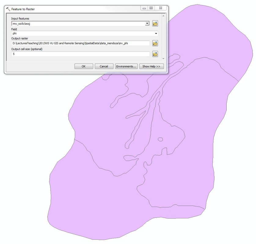
Making the joined colums permanent by exporting the data to a new shapefile (left and middle), conversion of the shape files of soil and land cover classes to raster maps (middle and right, only one example is shown as all of the resulting raster maps look similar).
Now join the land cover data table mv_lcovclass.txt to the land cover map mv_lcovclass.shp, again using the CLASS column as identifier. As you did it for the soil class map, make the joined table columns permanent by exporting the data to a new shapefile and prepare raster maps of root cohesion c_r and rooting depth d_r.

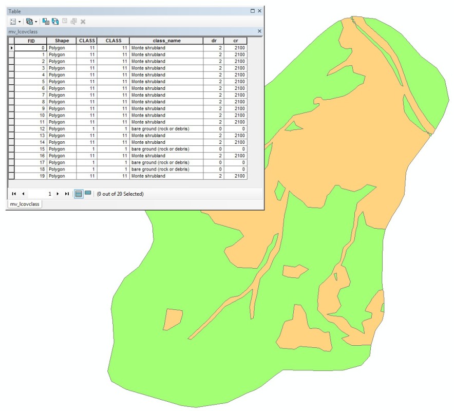
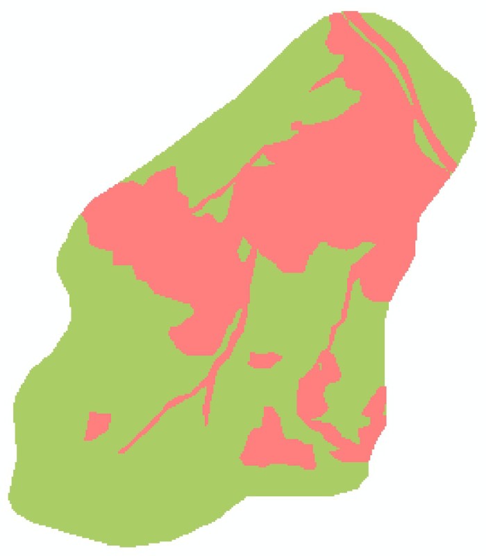
Joining the data assigned to each land cover class to the attribute table of the land cover class map (left) and - after making the joined columns of the attribute table permanent - converting the shape file into a raster (result on the right side, only shown for one parameter as the maps c_r and d_r look similar).
Before starting with the slope stability model, it is convenient to bring all maps to the units needed. The slope S and φ are needed in radian (now it is given in degree), θ_s is needed as fraction of the total volume (now it is given in per cent of volume).

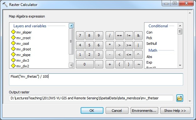
Conversion of the slope S (left) and saturated water content θ_s (right) rasters into units facilitating computing the factor of safety.

Now you have all the data ready to compute the Factor of Safety (FS) according to the infinite slope stability model. Slope stability strongly depends on soil water movement. We will compute slope stability first for dry soil, and then for fully saturated soil assuming slope-parallel water movement.

Principle of the infinite slope stability model.

First, calculate the factor of safety assuming dry soil (d_w = d_w,1) and a slip surface at d = 1 m. Don't forget to check the rooting depth: only if the roots reach deeper than the assumed slip surface, you may include root cohesion in the calculation. It is recommended to first compute rasters of the weight of moist soil W_m, and then, in a second step, the factor of safety. This helps to keep the expressions used clear.

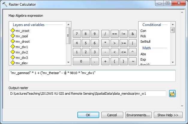
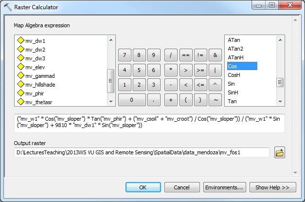
ArcMap raster calculator: expressions for W_m (left) and the factor of safety.
Repeat the calculation, assuming fully saturated soil (γ_w = 9810 N/m�, d = 1 m, d_w = d_w,2).
Finally, repeat the computation with fully saturated soil and d = 3 m (d_w = d_w,3).
Compare the result of each calculation to the slope failures observed in the field mv_init.shp.

Factor of safety for the three assumptions of soil water status and slip surface depth.

You will see that the result of the computation strongly depends on the assumptions of slip surface depth and the water status. Further, the outcomes strongly depend on the geotechnical parameters fed into the model. Careful field work, laboratory analysis and scenario-building are therefore highly important. Without good input data, even the most sophisticated GIS methods only produce colourful maps without any reliable information. In general, the interpretation of model results concerning hazardous processes is a highly critical task which requires extreme care and a lot of experience.

Various software packages exist coupling the infinite slope stability model to models of slope hydraulics, e.g. SINMAP or SHALSTAB.