Lesson 2: Working with terrain data and satellite imagery 2
1. Retrieval and preparation of data
For this lesson, we will use the SRTM DEM, the ASTER GDEM, Landsat 5 imagery and EO-1 imagery. All the data can be retrieved for free from CGIAR-CSI or from the Earth Explorer or downloaded directly from this site. The name of the SRTM DEM is srtm_51_05.tif, the name of the ASTER GDEM is ASTGTM2_N36E074_dem.tif. The Landsat 5 image L5149035_03520090827_***.TIF is from August 27, 2009. The file names of the EO-1 images do not reflect the date of acquisition:
- EO1A1490352010075110KF is from March 16, 2010;
- EO1A1490352010183110PF is from July 2, 2010;
- EO1A1490352010235110KF is from August 23, 2010.
The area of interest is defined by the polygon hz_extent.shp.
The preparation of the datasets works analogous to Lesson 1. Please project the SRTM DEM and the ASTER GDEM in a way to fit to the satellite imagery and clip all the data to the area of interest, as you have learned it in Lesson 1. The extent is not completely covered by the ASTER GDEM, a fact that does not matter in this specific case. Produce hillshades from both DEMs for a visual impression of the terrain and to see the differences between the two datasets. Next, produce false-colour composites of the satellite images. For the EO-1 imagery, use the channel combination 6-5-4 since the naming convention of the channels differs from that applied for the Landsat imagery. Then you have a dataset ready to be used for the analysis. Try to do a visual comparison of the images and interprete the changes you detect.
Learn more about GIS and RS data sources
Download training data for the Hunza Valley
2. Definition of the problem
When comparing the Landsat and EO-1 imagery, you will see that a lake was forming during the first half of 2010. This lake was dammed by a large landslide blocking the valley. This type of dam is prone to failure, leading to sudden drainage of the lake and major floods in the valley downstream.


Lake development illustrated by a series of three satellite images (from left to right: Landsat 5 from August 27, 2009 and EO-1 from March 16 and August 23, 2010).
In order to know about the potential magnitude of the event and to allow for efficient mitigation measures, the following knowledge is required:
- properties and stability of the dam. Even though high-resolution imagery can help to do so, this is a point where solely the application of GIS is insufficient, but field work and laboratory analysis are required.
- Volume of the lake, i.e. the maximum amount of water subjected to sudden drainage.
- Topography of the valley downstream, in order to know which are susceptible to be hit by a flood wave and how the flood wave behaves
The latter two tasks can be performed using GIS and remote sensing.
3. Derivation of lake volume
In order to estimate the volume of the lake, you must first integrate the dam in the DEM (except if you have a new DEM taken after the landslide). In most cases it will be sufficient to create a simplified dam body, the most important thing being the lowest point of the dam crest, i.e. the maximum lake level. There are various possibilities to create the dam, one of them is outlined here:
- Create a polygon feature in the same coordinate system as the preprocessed SRTM DEM. The polygon feature should be congruent with the dam identified in the satellite imagery. In direction perpendicular to the valley, it should reach over the actual dam. You can also use the dam polygon hz_dam.shp provided along with the other data.
- Convert the polygon feature into a raster with the same extent and resolution as the preprocessed SRTM DEM. For convenience, cells of the dam should have the value of the elevation of the dam, all other areas a value of 0. The elevation of the dam is very critical. in our case, it was measured in the field with 2420 m.

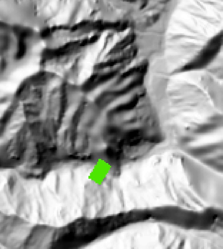
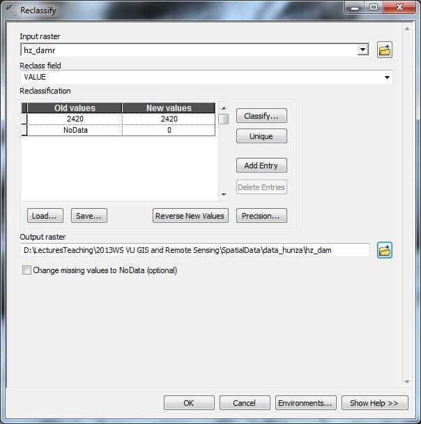

Conversion of the dam polygon (left) into a raster dataset (left middle) and converting no data cells to 0 (right middle and right). - Now combine the preprocessed SRTM DEM and the dam raster: for all cells where the dam raster has higher values than the DEM, the values of the dam raster are used. The DEM values are used for all the other cells.
- Ceate a hillshade of the modified DEM in order to see whether the dam has been added properly.
- Fill the sinks in the modified DEM. The area upsteam of the dam will be filled up to the dam level. Also, fill the sinks in the original DEM in order to remove artificial sinks and to make the original DEM comparable to the modified DEM.
Learn how to fill sinks in GRASS GIS 6.4, in ArcGIS 9.3 and in ArcGIS 10
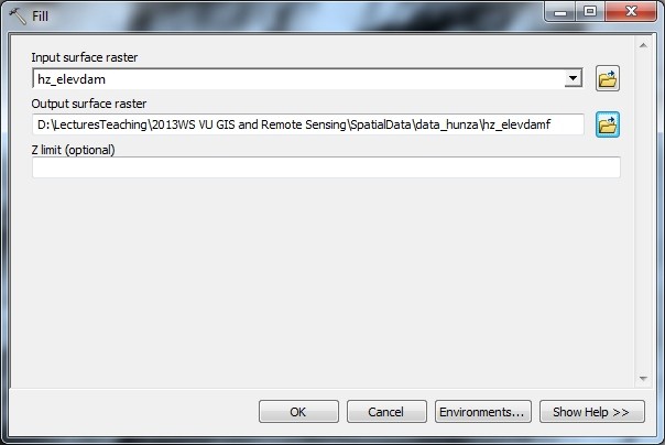

Filling of the elevation model - the hillshade nicely reveals the lake surface. - Subtract the modified DEM from the filled DEM in order to get the spatial distribution of lake depth.
- Finally, compute the volume from the depth distribution.
- Compare the depth distribution with the EO-1 image of August 2010 (when the lake was completely filled) in order to verify the result.
- Repeat all the previous steps with the ASTER GDEM and compare the results with those yielded using the SRTM DEM.
- Fill the sinks in the DEM. This is necessary to later compute consistent flow accumulation patterns.
- Compute the flow direction, i.e. the direction (N, NW etc.) in which a raster cell drains, from the filled DEM.
Learn how to compute the flow direction in GRASS GIS 6.4, in ArcGIS 9.3 and in ArcGIS 10
- From the flow direction raster, compute the flow accumulation. It denotes the number of cells draining through each cell.
Learn how to compute the flow accumulation in GRASS GIS 6.4, in ArcGIS 9.3 and in ArcGIS 10
- The main river is characterized by very high values of flow accumulation. By querying the map, define a lower threshold of what you would like to define as main river.
- Reclassify the flow accumulation raster map, with all cells defined as main river=1 and all other cells=no data.
- Convert the reclassified rater to a line feature. If necessary, remove trunks of lateral streams from the dataset.
Learn how to convert a raster map to line features in GRASS GIS 6.4, in ArcGIS 9.3 and in ArcGIS 10
- First, convert the vertices of the stream polyline to point features as you have learned in Lesson 1.
- Then apply the values of the DEM to these points by converting them into 3D features.
Learn how to convert 2D to 3D features in GRASS GIS 6.4, in ArcGIS 9.3 and in ArcGIS 10
- Add the elevation to the attribute table of the shape file. This step is actually not really necessary, but a good test whether the conversion has worked properly.
Learn how to add the z coordinate to a shapefile's attribute table in ArcGIS 9.3 and in ArcGIS 10
- Interpolate the point features to a raster as learned in Lesson 1. When using ArcGIS 9.3, in contrast to Lesson 1 you should use the Inverse Distance Weighted interpolation method directly from the Spatial Analyst (not from the ArcToolbox) and set the Analysis Extent to the area of interest before. Otherwise, the interpolation would not fill the entire area. When using ArcGIS 10, you can set the analysis extent in the ArcToolbox before running the interpolation.
- Finally, subtract the interpolated raster from the DEM.


Point feature representing the vertices of the valley bottom polyline (left), assigning elevation values to the points (left and middle) and interpolating the points to a raster surface (right). The dialog box in the right image shows how to overlay the interpolated raster surface with the digital elevation model in order to derive the height above river. - In order to facilitate the identification of highly critical areas, you can overlay the resulting raster map with a dataset of infrastructures and buildings. Such a dataset can be derived from the relevant agencies or mapped from remotely sensed data. Here you can use the polygon shapefile of cultivated areas (including farmland and settlements, but no roads or power lines) hz_cultivated.shp downloaded along with the other data.
- Particularly in narrow valleys sections and when using coarse DEMs, there may be artificial swells in the valley bottom (if the bottom is narrower than the DEM cell size). When filling the sinks, such swells are considered as dams and the area behind is filled up. Even though it would be much more realistic to "cut" the swells instead of filling up the areas behind, this would require complex algorithms not being standard in GIS software packages. Therefore, when applying the above method, one has to figure out and to mark clearly where such effects could bias the results.
- The information generated by this method should only be considered as a very rough overview. More sophisticated modelling techniques are required in order to get a better picture of which areas could be hit and which are likely to remain unaffected. Some of these methods will be introduced in Lesson 3.
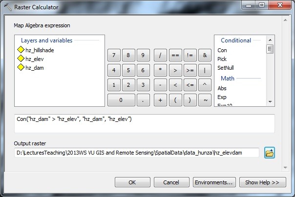
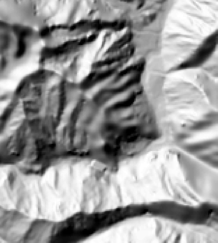
Analytic overlay of the DEM and the dam raster - the hillshade nicely illustrates the location of the dam.
Now you can compute the lake surface and compare the two surfaces in oder to derive the volume:
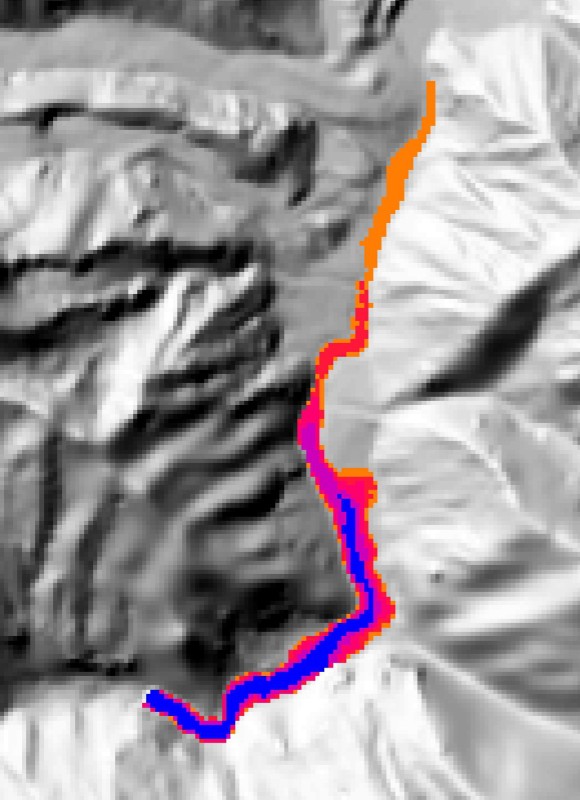
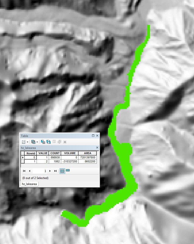
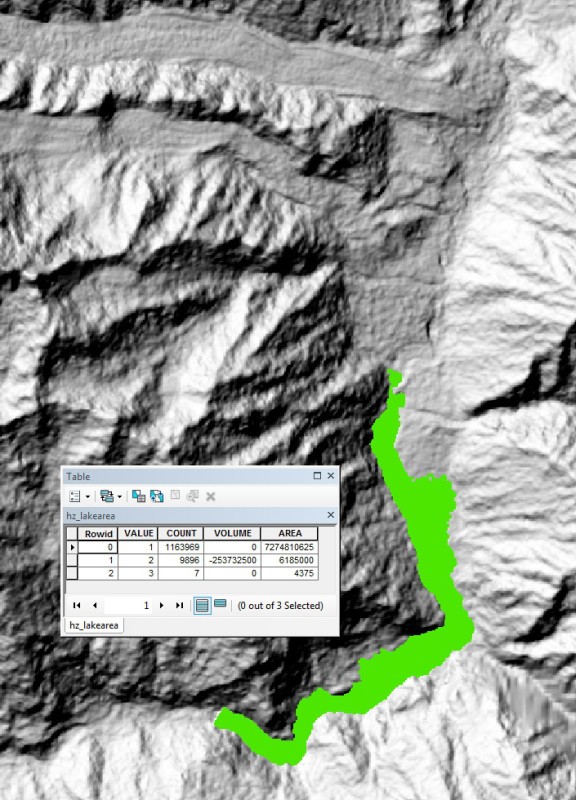
Derivation of lake depth distribution (left) and lake area and volume (middle) from the overlay of the original and the filled elevation models. The right image shows the lake area and volume derived from the ASTER GDEM following the same procedure. Even though the ASTER GDEM has a finer resolution and is better suited for a number of purposes, in this case it fails to reproduce the lake area due to an artefact affecting a narrow section of the valley.
4. Computation of height above valley bottom
The degree to which people, buildings or roads are susceptible to be affected by floods or debris flows strongly depends on the height above valley bottom. Creating a map of this parameter can give a first impression on which areas are more susceptible than others and where mitigation measures are most urgent.
Use the preprocessed SRTM DEM. First you have to generate a hydrologically clean DEM and to define the main river:
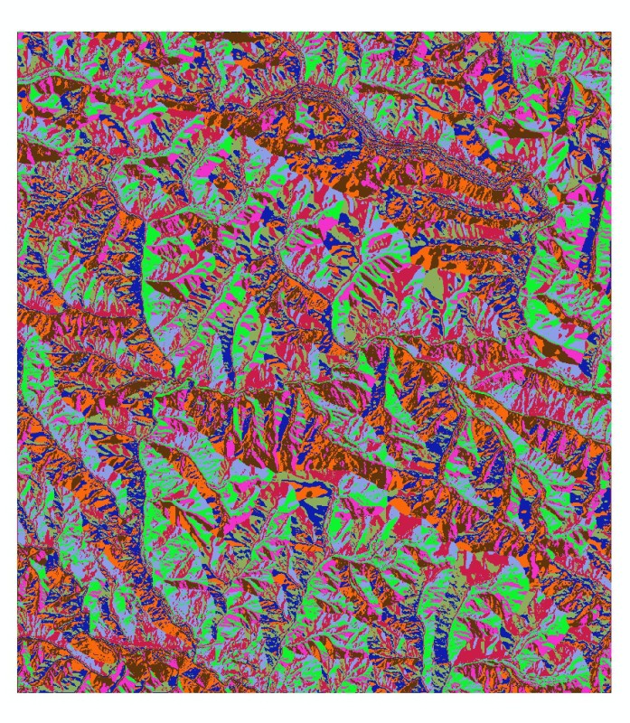
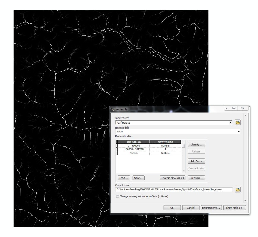

Flow direction (left) and flow accumulation rasters (middle). The raster map on the right side shows the reclassified flow accumulation raster with the dialog box for conversion into a line feature.
Now you have a line feature properly representing the main river or - more importantly - the valley bottom. You can derive the height of each cell of the DEM above the river (valley bottom). However, this does not work in a straightforward way:
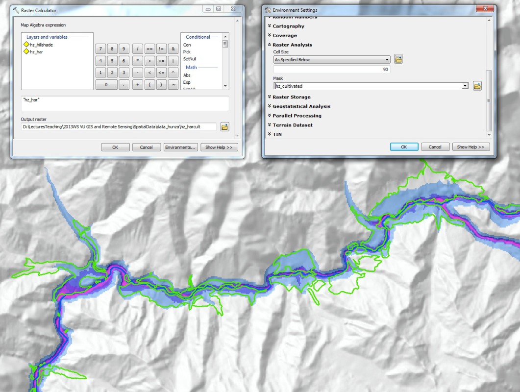
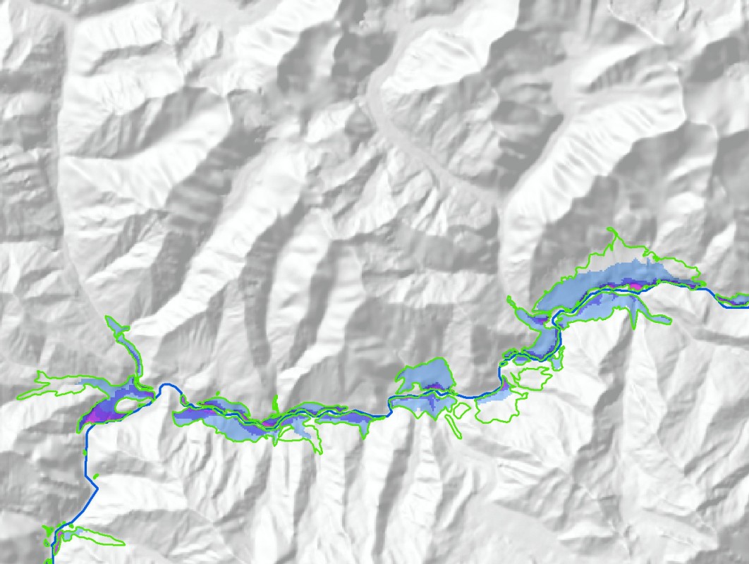
Height above river and borders of cultivated areas with dialog boxes for masking (left), height above river for cultivated areas (right).
There are at least two critical points to be considered: